
Tutorial Session in Week 04
Preparation
Before the class, you should make the following preparations:
- Bring your laptop (with a USB port)
- Configure the Python environment
- Prepare your favorite IDE
You can use Ubuntu (Recommended), Windows, or macOS for today’s workshop.
Below are the instructions for the Ubuntu system. For other systems, please search online for tutorials.
- Install Ubuntu on your computer
- Dual system installation(Recommended)
(https://www.bilibili.com/video/BV1554y1n7zv?p=1&vd_source=8a33bfef2a8deefbf13703472698cc56) - Virtual Machine Installation(May be some difficult problems to solve)
(https://blog.csdn.net/lhl_blog/article/details/123406322)
- Dual system installation(Recommended)
- Summary of commonly used shortcut keys in Ubuntu (https://blog.csdn.net/yzhang6_10/article/details/69569468)
Most commonly used commands
Ctrl + Alt + T:Open terminal
Ctrl + Shift + C:Copy in terminal
Ctrl + Shift + V:Paste in terminal- Install PyCharm+Annaconda environment (Optional but recommended)
- Anaconda install & common commands (https://blog.csdn.net/m0_50117360/article/details/108403586)
- Pycharm install in Ubuntu (https://blog.csdn.net/liangjian990709/article/details/112123533)
- Setting Anaconda in PyCharm (https://blog.csdn.net/liangjian990709/article/details/112123533)
- Programming environment on the right
conda create -n Me336Spring python=3.8
conda activate Me336Spring
# If installation fails, try using Tsinghua Source for installation
pip install opencv-python==4.4.0.46
# pip install opencv-python==4.4.0.46 -i https://pypi.tuna.tsinghua.edu.cn/simple
pip install opencv-contrib-python==4.4.0.46
# pip install opencv-contrib-python==4.4.0.46 -i https://pypi.tuna.tsinghua.edu.cn/simple
pip install numpy
# pip install numpy -i https://pypi.tuna.tsinghua.edu.cn/simple
pip install scikit-learn
# pip install scikit-learn -i https://pypi.tuna.tsinghua.edu.cn/simple
Class 1
A robotics engineer must learn computer vision, a crucial component in building and programming robots. Computer vision allows robots to perceive and interpret their surroundings through image processing and analysis, enabling them to make decisions, recognize objects and respond to environmental changes. Understanding computer vision enables a robotics engineer to design and develop more advanced and autonomous robots which can perform complex tasks and interact with their environment more effectively.
Image Acquisition
- Choose a device: digital cameras, webcams, and specialized machine vision cameras.
- Connect the device
- Configure the device: Configure the device settings, such as resolution, exposure time, and gain, to ensure that the images captured meet your needs.
- Acquire images: Use software or programming to acquire images from the device. This typically involves opening a connection to the device, specifying the settings, and capturing the images.
- Store the images: Store the images on your computer or another storage device for further processing and analysis.
- An example is shown on the right.
import cv2

# Initialize camera
cap = cv2.VideoCapture(0)

# Check if camera opened successfully
if not cap.isOpened():
    print("Error opening video capture")
    exit()

# Set camera properties (optional)
cap.set(cv2.CAP_PROP_FRAME_WIDTH, 1280)
cap.set(cv2.CAP_PROP_FRAME_HEIGHT, 720)
# cap.set(cv2.CV_CAP_PROP_FPS, 30);
# cap.set(cv2.CV_CAP_PROP_BRIGHTNESS, 1);
# cap.set(cv2.CV_CAP_PROP_CONTRAST,40);
# cap.set(cv2.CV_CAP_PROP_SATURATION, 50);
# cap.set(cv2.CV_CAP_PROP_HUE, 50);
# cap.set(cv2.CV_CAP_PROP_EXPOSURE, 50);

while True:
    # Capture frame-by-frame
    ret, frame = cap.read()

    # Display the resulting frame
    cv2.imshow('Camera', frame)

    # Wait for key press
    key = cv2.waitKey(1) & 0xFF

    # Check if 's' key is pressed to save image
    if key == ord('s'):
        cv2.imwrite('image.jpg', frame)
        print("Image captured!")
        break

# Release the camera and close all windows
cap.release()
cv2.destroyAllWindows()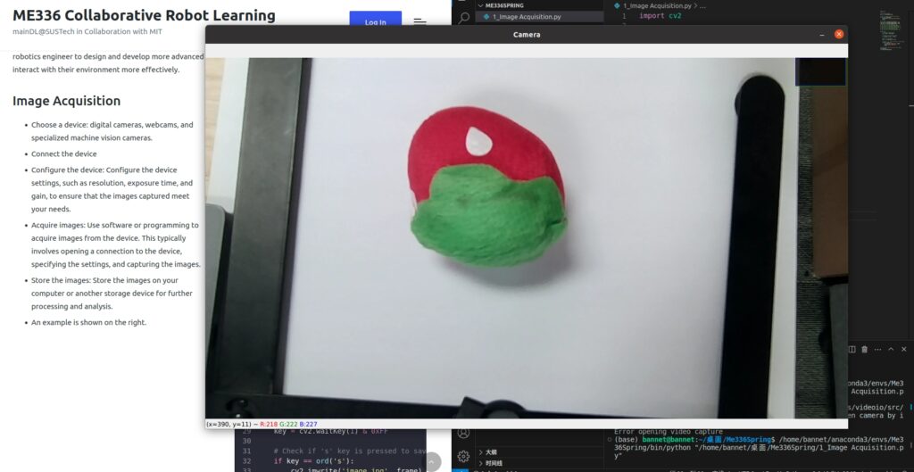
Image Pre-processing
Image pre-processing is a crucial step in machine vision, as it can significantly impact the accuracy and performance of the final results. It is crucial to choose the proper pre-processing techniques for the specific application and to use them judiciously to avoid distorting the original information in the image.It typically involves several steps to clean up and enhance the images.
Noise Reduction
- Removing noise or random fluctuations in the image data to improve the quality and accuracy of the image.
- For the example on the right
- This code first loads an image using OpenCV’s
imreadfunction and applies a Gaussian blur usingGaussianBlurto reduce noise. The resulting filtered image is then displayed usingimshow. - The Gaussian blur is a popular method for noise reduction in images. It replaces each pixel value in the image with the weighted average of its neighboring pixels, effectively smoothing the image and reducing high-frequency noise. The size of the Gaussian kernel and the standard deviation can be adjusted to control the amount of smoothing applied to the image.
- This code first loads an image using OpenCV’s
import cv2

# Load the image
img = cv2.imread('image.jpg')

# Apply Gaussian filter
filtered = cv2.GaussianBlur(img, (5, 5), 0)

# Display the original and filtered images side by side
cv2.imshow('Original', img)
cv2.imshow('Filtered', filtered)
cv2.waitKey(0)
cv2.destroyAllWindows()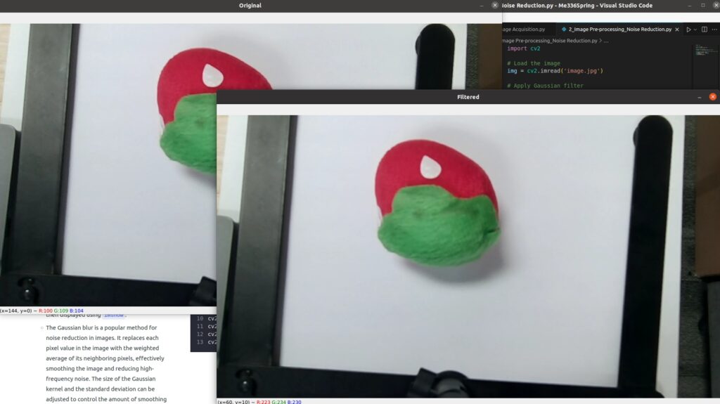
Image Correction
- Correcting issues such as color cast or distortion in the image.
- For the example on the right
- This code first loads an image using OpenCV’s
imreadfunction, then convert the image to YUV color space usingcv2.cvtColor()function, and applies histogram equalization usingequalizeHistto correct the color balance. The corrected image is then converted back to the original color space usingcvtColorand displayed usingimshow. - You can adjust the parameters of the histogram equalization function to achieve the desired correction. Additionally, you can also apply histogram equalization to other color spaces such as HSV, LAB, or LCH to correct color balance.
- This code first loads an image using OpenCV’s
import cv2

# Load the image
img = cv2.imread('image.jpg')

# Apply histogram equalization to each color channel
equalized = cv2.cvtColor(img, cv2.COLOR_BGR2YUV)
equalized[:, :, 0] = cv2.equalizeHist(equalized[:, :, 0])
equalized = cv2.cvtColor(equalized, cv2.COLOR_YUV2BGR)

# Display the original and equalized images side by side
cv2.imshow('Original', img)
cv2.imshow('Equalized', equalized)
cv2.waitKey(0)
cv2.destroyAllWindows()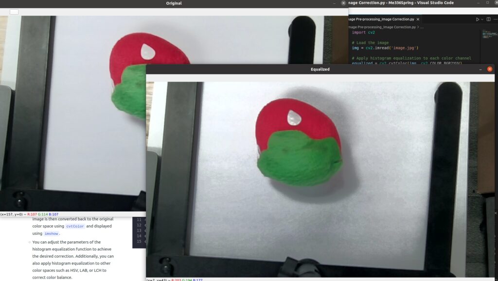
Image Enhancement
- Improving the visibility of features in the image, such as increasing contrast or sharpness.
- For the example on the right
- This code first loads an image using OpenCV’s
imreadfunction, converts it to grayscale usingcvtColor, and applies histogram equalization usingequalizeHistto enhance the contrast. The resulting enhanced image is then displayed usingimshow. - Histogram equalization is a simple yet effective method for image enhancement. It adjusts the distribution of pixel values in an image to improve the image contrast. This can make features in the image more visible and easier to distinguish, which can be particularly useful for images with low contrast or poor lighting conditions.
- This code first loads an image using OpenCV’s
import cv2
import numpy as np

# Load the image
img = cv2.imread('image.jpg')

# Convert the image to grayscale
gray = cv2.cvtColor(img, cv2.COLOR_BGR2GRAY)

# Apply a histogram equalization to enhance the image contrast
enhanced = cv2.equalizeHist(gray)

# Show the original and enhanced images
cv2.imshow('Original Image', gray)
cv2.imshow('Enhanced Image', enhanced)
cv2.waitKey(0)
cv2.destroyAllWindows()
Image Segmentation
- Partitioning an image into multiple regions corresponds to a different object or background.
- For the example on the right
- This code first loads an image using OpenCV’s
imreadfunction, converts it to grayscale usingcvtColor, and applies thresholding usingthresholdto segment the image into foreground and background regions. The resulting thresholded image is then displayed usingimshow. - Thresholding is a simple yet effective method for image segmentation. It converts an image into a binary image by setting all pixels above a specified threshold to the maximum value (255) and all pixels below the threshold to the minimum value (0 in this case). This effectively separates the image into foreground and background regions, making it easier to identify objects or features in the image. The threshold value can be adjusted to control the level of detail in the segmented image.
- This code first loads an image using OpenCV’s
import cv2
import numpy as np

# Load the image
img = cv2.imread('image.jpg')

# Convert the image to grayscale
gray = cv2.cvtColor(img, cv2.COLOR_BGR2GRAY)

# Apply thresholding to segment the image
_, thresholded = cv2.threshold(gray, 128, 255, cv2.THRESH_BINARY)

# Show the original and thresholded images
cv2.imshow('Original Image', img)
cv2.imshow('Thresholded Image', thresholded)
cv2.waitKey(0)
cv2.destroyAllWindows()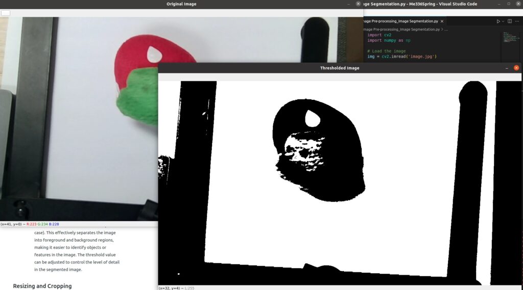
Resizing and Cropping
- Changing the size or aspect ratio of the image or removing unwanted regions from the image.
- For the example on the right
- This code first loads an image using OpenCV’s
imreadfunction, resizes it using resize to a specific size (600×400 pixels in this case), and crops it using indexing to a specific region (100 to 300 pixels in the vertical direction and 200 to 400 pixels in the horizontal direction in this case). The original, resized, and cropped images are then displayed usingimshow. - Resizing and cropping are common pre-processing steps for images in computer vision and image processing. Resizing can be used to change the size of an image, which can be important for image processing algorithms that require a specific size or aspect ratio. Cropping can extract a particular region of interest from an image, which can help remove unwanted parts of an image or focus on specific features.
- This code first loads an image using OpenCV’s
import cv2
import numpy as np

# Load the image
img = cv2.imread('image.jpg')

# Resize the image
resized = cv2.resize(img, (600, 400), interpolation=cv2.INTER_AREA)

# Crop the image
cropped = resized[100:300, 200:400]

# Show the original, resized, and cropped images
cv2.imshow('Original Image', img)
cv2.imshow('Resized Image', resized)
cv2.imshow('Cropped Image', cropped)
cv2.waitKey(0)
cv2.destroyAllWindows()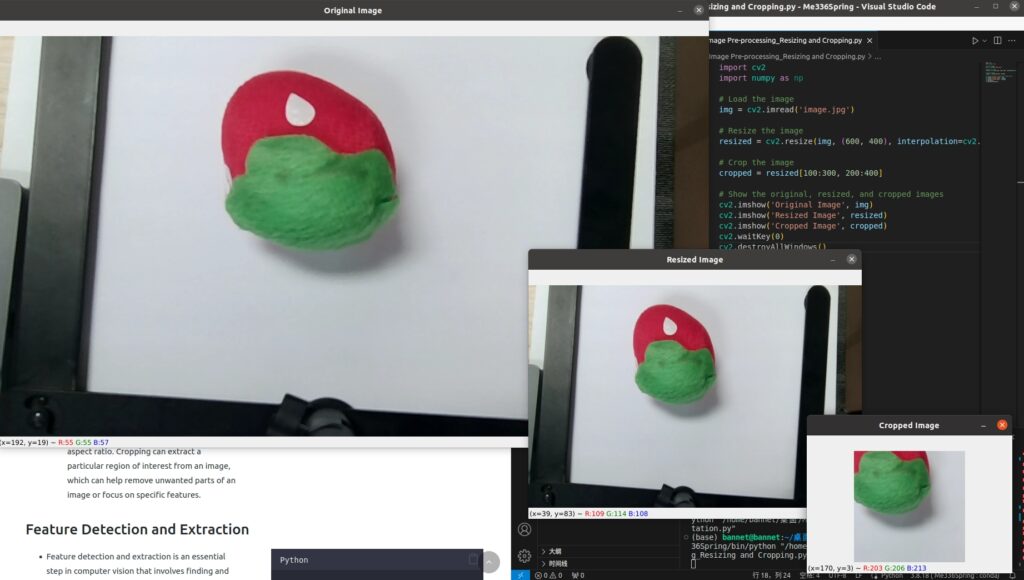
Feature Detection and Extraction
- Feature detection and extraction is an essential step in computer vision that involves finding and describing the key points or features in an image that are relevant to a specific task, such as object recognition, image matching, or tracking. There are many different feature detection and extraction algorithms, each with strengths and weaknesses, depending on the specific task and the type of image.
- Shown on the right is an example of feature detection and extraction in Python using the OpenCV library and the SIFT (Scale-Invariant Feature Transform) algorithm.
- This code first loads an image using OpenCV’s
imreadfunction, converts it to grayscale usingcvtColor, and creates a SIFT object usingcv2.SIFT_create. ThedetectAndComputefunction is then used to detect key points in the image and compute their descriptors. The resulting key points are drawn on the image usingdrawKeypoints, and the original and keypoint-annotated images are displayed usingimshow. - SIFT is a popular feature detection and extraction algorithm that is robust to image scale, orientation, and affine distortion. It works by detecting distinctive points in an image and computing a descriptor that describes the local appearance of the image at that point. The descriptors can then be used for tasks such as image matching, object recognition, or tracking. The key points and descriptors can also be visualized on the image to help understand and debug.
- This code first loads an image using OpenCV’s
import cv2

# Load the input image
input_image = cv2.imread('image.jpg')

# Convert the input image to grayscale
gray_image = cv2.cvtColor(input_image, cv2.COLOR_BGR2GRAY)

# Create a SIFT object for feature detection and extraction
sift = cv2.SIFT_create()

# Detect keypoints and compute descriptors for the input image
keypoints, descriptors = sift.detectAndCompute(gray_image, None)

# Draw the detected keypoints on the input image
output_image = cv2.drawKeypoints(input_image, keypoints, None)

# Show the output image
cv2.imshow('Output Image', output_image)
cv2.waitKey(0)
cv2.destroyAllWindows()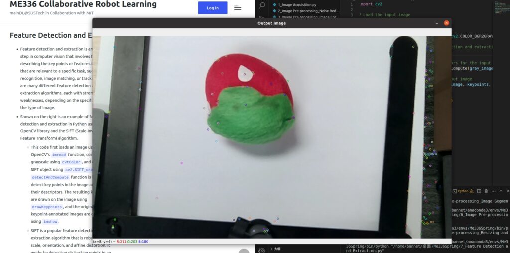
Image Analysis and Interpretation
- Image analysis and interpretation extract meaningful information and insights from images. It involves a combination of computer vision techniques, such as feature detection and extraction, image segmentation, and machine learning, to understand the content of an image and make decisions based on that information.
- For example, an image analysis and interpretation system could detect and classify objects in an image, recognize handwritten text, analyze medical images for signs of disease, or interpret satellite images for environmental monitoring.
- Here is an example of image analysis and interpretation for shape detection:
- This code creates a window called ‘Canvas’, and sets up a mouse callback function that draws on the canvas when the left mouse button is pressed and dragged. When the mouse button is released, the code converts the canvas to grayscale, thresholds it, finds the contours, and identifies the shape of the outline by checking the number of corners using
cv2.approxPolyDP(). Finally, the code displays the canvas on the screen and prints the final shape when the user presses the ‘q’ key.
- This code creates a window called ‘Canvas’, and sets up a mouse callback function that draws on the canvas when the left mouse button is pressed and dragged. When the mouse button is released, the code converts the canvas to grayscale, thresholds it, finds the contours, and identifies the shape of the outline by checking the number of corners using
import cv2
import numpy as np
# Set up the canvas
canvas = np.zeros((480, 640, 3), dtype=np.uint8)
drawing = False
ix, iy = -1, -1
shape = ''
# Define the mouse callback function
def draw_shape(event, x, y, flags, param):
global canvas, drawing, ix, iy, shape
if event == cv2.EVENT_LBUTTONDOWN:
drawing = True
ix, iy = x, y
elif event == cv2.EVENT_MOUSEMOVE:
if drawing == True:
cv2.line(canvas, (ix, iy), (x, y), (0, 0, 255), 2)
ix, iy = x, y
elif event == cv2.EVENT_LBUTTONUP:
drawing = False
cv2.line(canvas, (ix, iy), (x, y), (0, 0, 255), 2)
# Convert the canvas to grayscale and threshold it
gray = cv2.cvtColor(canvas, cv2.COLOR_BGR2GRAY)
_, thresh = cv2.threshold(gray, 10, 255, cv2.THRESH_BINARY)
# Find contours in the thresholded image
contours, _ = cv2.findContours(thresh, cv2.RETR_EXTERNAL, cv2.CHAIN_APPROX_SIMPLE)
# Identify the shape of the outline
for cnt in contours:
area = cv2.contourArea(cnt)
if area < 500:
# Ignore small contours
continue
peri = cv2.arcLength(cnt, True)
approx = cv2.approxPolyDP(cnt, 0.04 * peri, True)
if len(approx) == 3:
shape = 'Triangle'
elif len(approx) == 4:
shape = 'Rectangle'
else:
shape = 'Circle'
# Set up the window and mouse callback
cv2.namedWindow('Canvas')
cv2.setMouseCallback('Canvas', draw_shape)
# Main loop
while True:
cv2.imshow('Canvas', canvas)
key = cv2.waitKey(1) & 0xFF
if key == ord('q'):
break
elif key == ord('c'):
canvas = np.zeros((480, 640, 3), dtype=np.uint8)
shape = ''
# Print the final shape
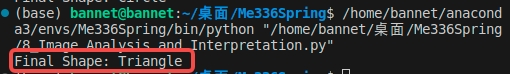
print('Final Shape: {}'.format(shape))
cv2.destroyAllWindows()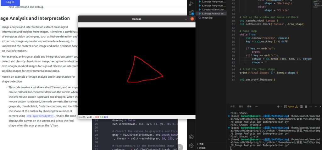
Feedback and Control
- Machine vision systems often provide feedback to control other systems, such as robots, to perform tasks based on the visual information they receive.
Operational Efficiency
- Software operational efficiency is critical in computer vision as it can impact the performance and speed of computer vision systems and applications. An efficient computer vision system will quickly process images and video frames, which is critical for real-time applications. Inefficient systems can lead to slow processing times, high memory usage, and reduced accuracy, impacting overall performance and user experience.
- Take two methods for tracking human faces in real-time as an example.
- Sample Method 1: This code uses the
haarcascade_frontalface_default.xmlclassifier from OpenCV’s pre-trained Haar cascades to detect faces in the video frames. The rectangles around the detected faces are drawn in real-time and displayed in a window namedFrame. - Sample Method 2: In this example, the
face_cascadeis a trained Haar cascade classifier for face detection, which is loaded from a file. Thecapobject is used to capture the video frames from the default camera. Theface_rectvariable stores the initial window for the face ROI, which is updated in each iteration of the loop using theMOSSE trackerfunction.
- Sample Method 1: This code uses the
- Model File (Click to Download)
import cv2
import time

# Load the pre-trained classifier
face_cascade = cv2.CascadeClassifier('haarcascade_frontalface_default.xml')

# Initialize the video capture device
cap = cv2.VideoCapture(0)
cap.set(cv2.CAP_PROP_FRAME_WIDTH, 1280)
cap.set(cv2.CAP_PROP_FRAME_HEIGHT, 720)
# Initialize variables for calculating average time
total_time = 0
frame_count = 0

while True:
    # Capture frame-by-frame and record start time
    ret, frame = cap.read()
    start_time = time.time()

    # Convert the frame to grayscale
    gray = cv2.cvtColor(frame, cv2.COLOR_BGR2GRAY)

    # Detect faces in the grayscale frame
    faces = face_cascade.detectMultiScale(gray, scaleFactor=1.1, minNeighbors=5)

    # Draw a rectangle around each detected face
    for (x, y, w, h) in faces:
        cv2.rectangle(frame, (x, y), (x + w, y + h), (0, 255, 0), 2)

    # Display the resulting frame
    cv2.imshow('frame', frame)

    # Calculate time spent on this frame and update variables
    end_time = time.time()
    time_spent = end_time - start_time
    total_time += time_spent
    frame_count += 1

    # Check for key press and exit if necessary
    if cv2.waitKey(1) & 0xFF == ord('q'):
        break

# Release the capture device and close all windows
cap.release()
cv2.destroyAllWindows()

# Calculate and print average time spent per frame
avg_time_per_frame = total_time / frame_count
print("Average time spent per frame: {:.2f} seconds".format(avg_time_per_frame))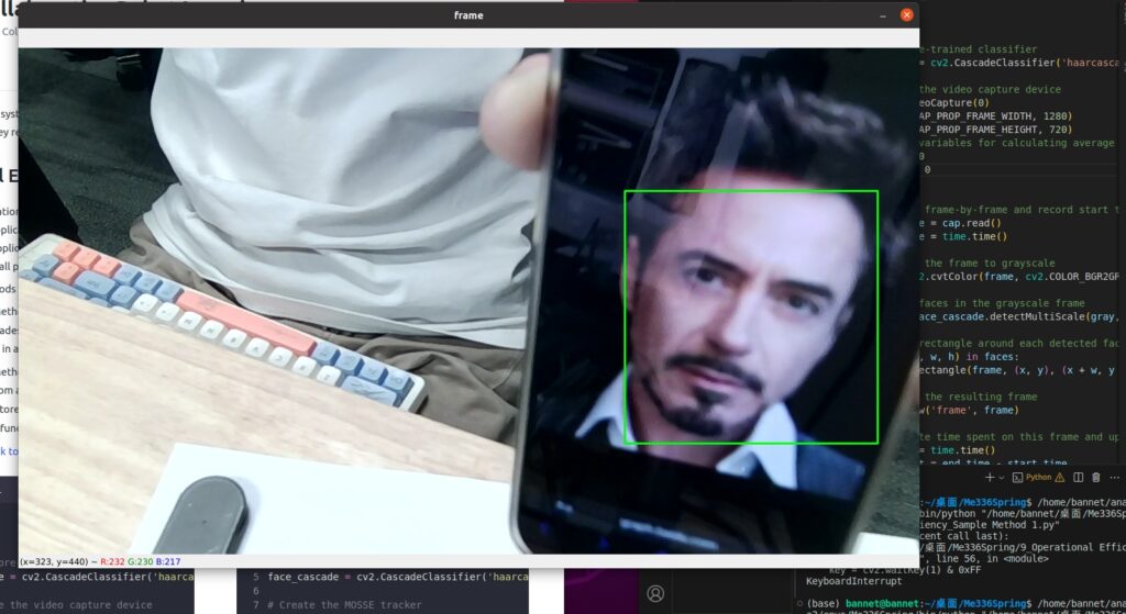
import cv2
import time

# Load the pre-trained Haar Cascade classifier
face_cascade = cv2.CascadeClassifier('haarcascade_frontalface_default.xml')

# Create the MOSSE tracker
tracker = cv2.TrackerMOSSE_create()

# Load the video
cap = cv2.VideoCapture(0)
cap.set(cv2.CAP_PROP_FRAME_WIDTH, 1280)
cap.set(cv2.CAP_PROP_FRAME_HEIGHT, 720)
# Initialize variables for time measurement
frame_count = 0
total_time = 0

# Read the first frame
ret, frame = cap.read()

# Detect the initial face(s) using the Haar Cascade classifier
gray = cv2.cvtColor(frame, cv2.COLOR_BGR2GRAY)
faces = face_cascade.detectMultiScale(gray, scaleFactor=1.3, minNeighbors=5)

# Initialize the tracker with the first face (if any)
if len(faces) > 0:
    # Select the first face
    (x, y, w, h) = faces[0]
    # Initialize the tracker with the first face
    tracker.init(frame, (x, y, w, h))

# Loop over each frame in the video
while True:
    # Read a frame from the video
    ret, frame = cap.read()
    # If we reached the end of the video, break out of the loop
    if not ret:
        break

    # Start the timer
    start_time = time.time()

    # Track the face using the MOSSE tracker (if initialized)
    if tracker:
        # Update the tracker with the current frame
        ok, bbox = tracker.update(frame)
        # If the tracking was successful, draw a rectangle around the face
        if ok:
            (x, y, w, h) = [int(v) for v in bbox]
            cv2.rectangle(frame, (x, y), (x + w, y + h), (0, 255, 0), 2)
        # If the tracking failed (e.g., the face went out of the frame), reset the tracker
        else:
            tracker = None

    # If the tracker is not initialized or failed, detect faces using the Haar Cascade classifier
    if not tracker:
        # Convert the frame to grayscale
        gray = cv2.cvtColor(frame, cv2.COLOR_BGR2GRAY)
        # Detect faces in the grayscale image using the Haar Cascade classifier
        faces = face_cascade.detectMultiScale(gray, scaleFactor=1.3, minNeighbors=5)
        # If a face is detected, initialize the tracker with the first face
        if len(faces) > 0:
            (x, y, w, h) = faces[0]
            tracker = cv2.TrackerMOSSE_create()
            tracker.init(frame, (x, y, w, h))

    # Show the frame with the detected/tracked face
    cv2.imshow('frame', frame)

    # Stop the timer and update the time variables
    end_time = time.time()
    total_time += end_time - start_time
    frame_count += 1

    # Wait for a key press, and exit the loop if the 'q' key is pressed
    if cv2.waitKey(1) & 0xFF == ord('q'):
        break

# Release the resources (camera and window)
cap.release()
cv2.destroyAllWindows()

# Calculate the average time cost per frame
average_time = total_time / frame_count
print('Average time cost per frame: {:.2f} seconds'.format(average_time))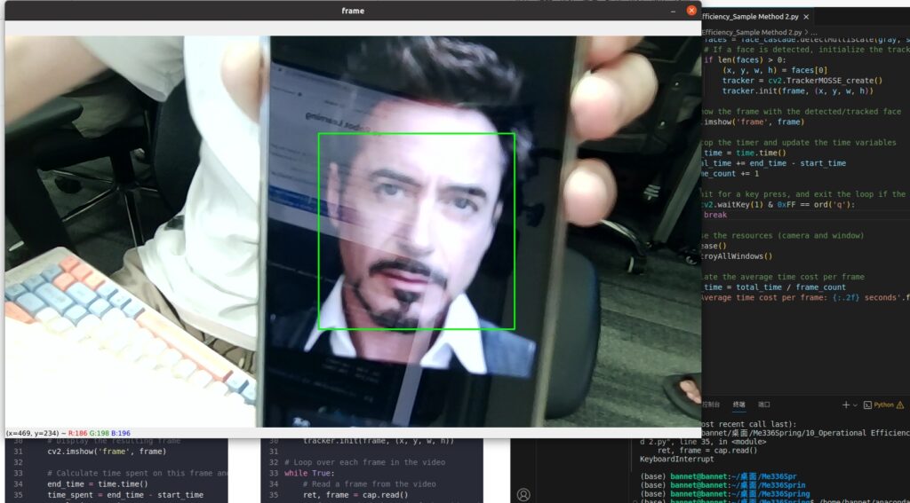
Class 2 on Mar 15th
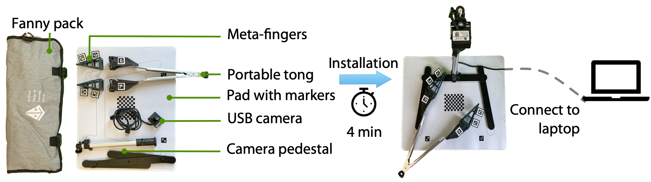
Hardware Toolkit
Part 1: Pose Estimation
- Pose estimation is the process of determining the position and orientation of an object in a given environment. It is commonly used in computer vision and robotics applications, such as human-computer interaction, augmented reality, and autonomous navigation. Pose estimation algorithms use a combination of computer vision techniques, such as feature detection, image segmentation, and machine learning, to estimate the position and orientation of an object in 3D space based on its image or a sequence of images. The accuracy of pose estimation results can be affected by various factors, such as the quality of the images, the complexity of the object, and the presence of occlusions.
Task 1: Camera Calibration
Camera calibration is essential before pose estimation because it helps correct the camera’s intrinsic and extrinsic parameters. These parameters include:
- Intrinsic Parameters: Characterize the camera’s internal optics and geometry, such as the focal length, principal point, and lens distortion.
- Extrinsic Parameters: Characterize the position and orientation of the camera about the world coordinate system, such as the position of the camera, its orientation, and the skew between the x and y axes
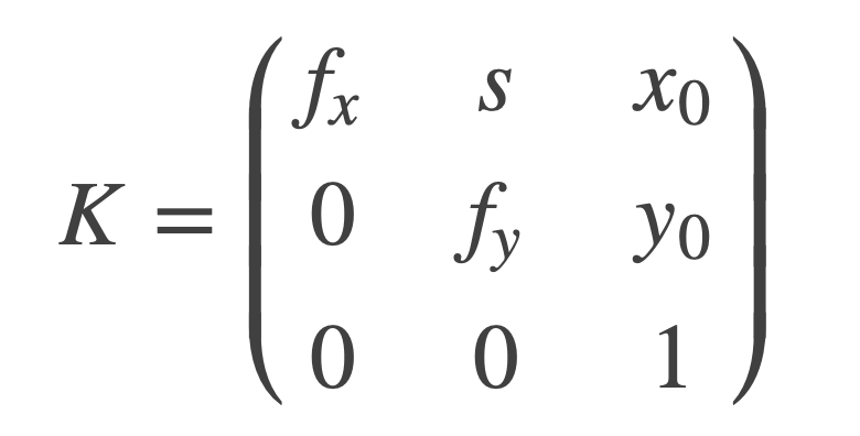
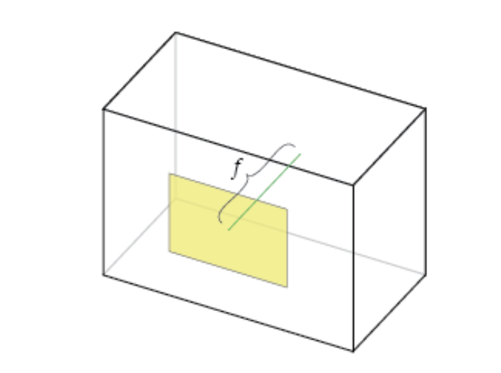
Focal Length, fx, fy:
The focal length is the distance between the pinhole and the film (a.k.a. image plane).
Axis Skew, s
Skew coefficient, which is non-zero if the image axes are not perpendicular.
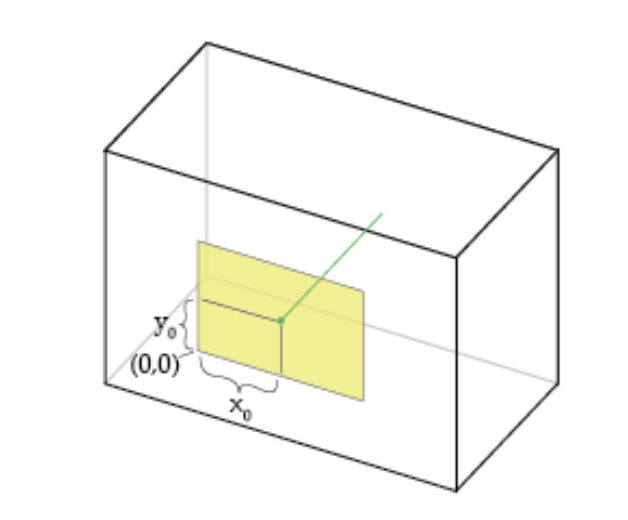
Principal Point Offset x0, y0:
The camera’s “principal axis” is the line perpendicular to the image plane that passes through the pinhole. Its itersection with the image plane is referred to as the “principal point,” illustrated below.
Without camera calibration, the estimated pose of the object would be incorrect due to the lens distortion, aspect ratio, and perspective effects introduced by the camera. Additionally, camera calibration helps to remove the effects of non-uniform illumination and other environmental factors that can affect the quality of the image data.
In the image below, the parameters of the lens estimated using geometric calibration were used to un-distort the image.
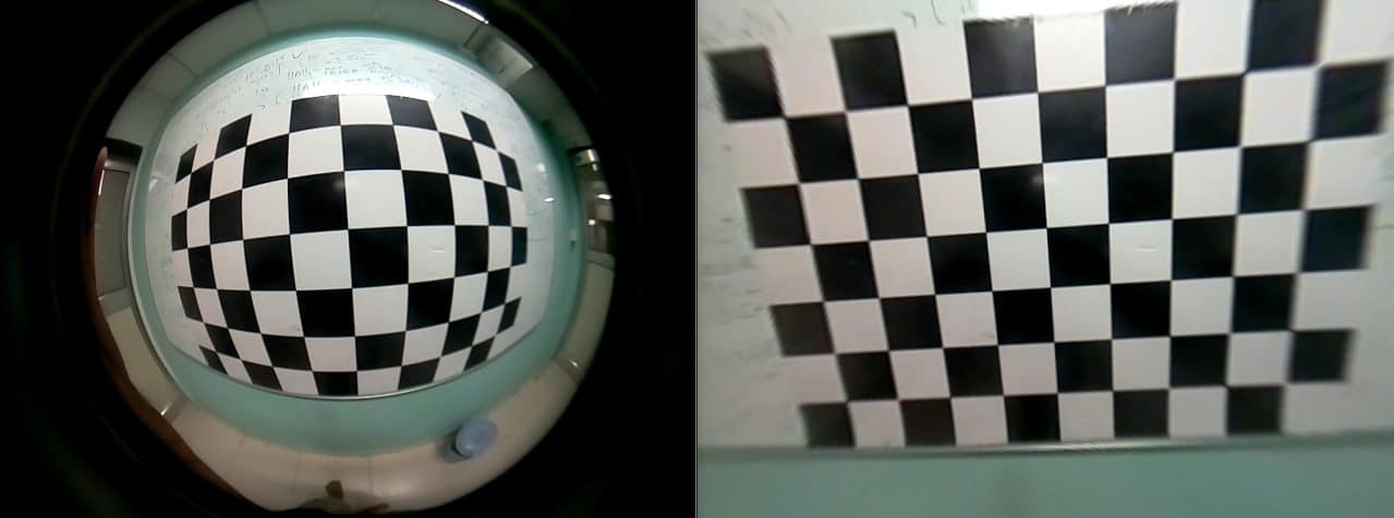
Camera calibration can be performed using a calibration pattern, such as a checkerboard pattern, and can be done offline or online, depending on the application’s requirements. Once the camera parameters are known, they can rectify the image, so the lines are parallel to the plane. These steps help improve the pose estimation accuracy and ensure that the estimated pose is reliable and repeatable. Click here to download calibration table mat.
You can learn more about camera calibration from the OpenCv documentation here.
Using the following code, you can complete the task of photographing and camera calibration. You first need to enter the camera serial number, in most cases it should be 0, if you can not open the USB camera, you can try to change to 1 or -1. Then, enter the number of photos you need to take, which is recommended to be around 20. Finally, you will get a file called ‘camera_params.npz’ which will store the parameters of the camera.
import cv2
import numpy as np
import os
import time
import shutil
import sys

# Set the chessboard size and grid width
num_horizontal = 11
num_vertical = 8
grid_width = 0.007    # meter

def capture_calibration_images(camera_id, num_images, delay=3):
    folder = 'cali_imgs'
    if os.path.exists(folder):
        # Delete all files in the folder
        for filename in os.listdir(folder):
            file_path = os.path.join(folder, filename)
            try:
                if os.path.isfile(file_path) or os.path.islink(file_path):
                    os.unlink(file_path)
                elif os.path.isdir(file_path):
                    shutil.rmtree(file_path)
            except Exception as e:
                print(f'Failed to delete {file_path}. Reason: {e}')
    else:
        # If the folder does not exist, create it
        os.makedirs(folder)

    cap = cv2.VideoCapture(camera_id)
    if not cap.isOpened():
        print("Failed to open the camera. Reason: {cap}")
        return

    photo_count = 0
    start_time = time.time()

    while cap.isOpened() and photo_count < num_images:
        ret, frame = cap.read()
        font = cv2.FONT_HERSHEY_SIMPLEX
        # Calculate the remaining time for the countdown (in seconds)
        current_time = time.time()
        elapsed_time = current_time - start_time
        remaining_time = delay - elapsed_time if elapsed_time < delay else 0

        # Calculate the end angle of the sector
        end_angle = 360 * remaining_time / delay

        # Create a copy of the original image with the same size
        overlay = np.zeros_like(frame)

        # Create a copy of the original image with the same size
        overlay = frame.copy()

        # Draw a white ellipse on the copy
        cv2.ellipse(overlay, (int(frame.shape[1]*0.5), int(frame.shape[0]*0.5)), (int(frame.shape[0]*0.5), int(frame.shape[0]*0.5)), -90, 0, end_angle, (255, 255, 255), -1)

        # Blend the copy and the original image with a transparency of 50%
        alpha = 0.5
        cv2.addWeighted(overlay, alpha, frame, 1 - alpha, 0, frame)
        cv2.putText(frame, f'Photo {photo_count + 1}/{num_images}', (frame.shape[1] - 200, frame.shape[0] - 10), font, 0.5, (0, 255, 0), 2, cv2.LINE_AA)
        cv2.imshow('Calibration', frame)

        # Break the loop if 'q' is pressed
        if cv2.waitKey(1) & 0xFF == ord('q'):
            break

        # Save the image every delay seconds
        if time.time() - start_time >= delay:
            filename = os.path.join(folder, f'image_{photo_count}.jpg')
            cv2.imwrite(filename, frame)
            print(f"Image saved:{filename}")
            photo_count += 1
            start_time = time.time()

            # After saving the image, display a white image
            white_frame = np.ones_like(frame) * 255
            cv2.imshow('Calibration', white_frame)
            cv2.waitKey(100)
            cv2.imshow('Calibration', frame)

    cap.release()
    cv2.destroyAllWindows()

def calibrate_camera(folder):
    # termination criteria
    criteria = (cv2.TERM_CRITERIA_EPS + cv2.TERM_CRITERIA_MAX_ITER, 30, 0.001)
    # prepare object points, like (0,0,0), (1,0,0), (2,0,0) ....,(10,7,0)
    objp = np.zeros((num_vertical*num_horizontal,3), np.float32)
    objp[:,:2] = np.mgrid[0:num_horizontal,0:num_vertical].T.reshape(-1,2) * grid_width
    # Arrays to store object points and image points from all the images.
    objpoints = [] # 3d point in real world space
    imgpoints = [] # 2d points in image plane.
    # Read images
    images = [os.path.join(folder, f) for f in os.listdir(folder) if f.endswith('.jpg')]
    images = sorted(images, key=lambda x: int(os.path.splitext(os.path.basename(x))[0].split('_')[1]))

    for fname in images:
        img = cv2.imread(fname)
        print("Image: ", fname)
        gray = cv2.cvtColor(img, cv2.COLOR_BGR2GRAY)
        # Find the chess board corners
        ret, corners = cv2.findChessboardCorners(gray, (num_horizontal, num_vertical), None)

        # If found, add object points, image points (after refining them)
        if ret == True:
            print('conership:', corners.shape[0])
            objpoints.append(objp)
            corners2 = cv2.cornerSubPix(gray, corners, (11,11), (-1,-1), criteria)
            imgpoints.append(corners2)
            # Draw and display the corners
            cv2.drawChessboardCorners(img, (num_horizontal, num_vertical), corners2, ret)
            cv2.imshow('img', img)
            cv2.waitKey(500)

    if not objpoints or not imgpoints:
        print("Not enough corners were detected for calibration")
        time.sleep(2)
        sys.exit(1)

    cv2.destroyAllWindows()

    # Calibrate the camera
    ret, mtx, dist, rvecs, tvecs = cv2.calibrateCamera(objpoints, imgpoints, gray.shape[::-1], None, None)

    # Calculate reprojection error
    mean_error = 0
    for i in range(len(objpoints)):
        imgpoints2, _ = cv2.projectPoints(objpoints[i], rvecs[i], tvecs[i], mtx, dist)
        error = cv2.norm(imgpoints[i],imgpoints2, cv2.NORM_L2)/len(imgpoints2)
        mean_error += error
    mean_error /= len(objpoints)
    print(f"Reprojection error: {mean_error}")

    # Check if calibration is qualified
    if mean_error < 1:
        np.savez("camera_params.npz", mtx=mtx, dist=dist, rvecs=rvecs, tvecs=tvecs)
        print("Camera calibrated")
    else:
        print("Calibration failed, please try again")

    return ret, mtx, dist, rvecs, tvecs

# Ask the user to input the camera ID
camera_id = int(input("Please enter your camera ID: "))
num_images = int(input("Please enter the number of photos you want to take: "))

capture_calibration_images(camera_id, num_images)

ret, mtx, dist, rvecs, tvecs = calibrate_camera('cali_imgs')
if ret:
    print("Calibration successful! Camera parameters are saved in 'camera_params.npz' file.")
    np.set_printoptions(precision=4, suppress=True)
    print('Camera Intrinsics Matrix:\n[[fx\t0\tcx]\n[0\tfy\tcy]\n[0\t0\t1]]  =\n', np.round(mtx, 4))
    print('dist:', np.round(dist, 4))
Task 2: Visual Object Tracking
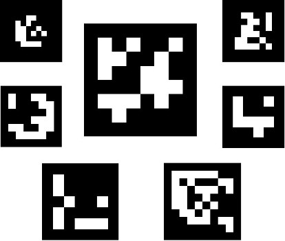
- In this part of the experiment, you will use the camera parameters obtained in the above steps and use them to estimate the 6D pose of ArUco marker and collect the data for further use.
- ArUco marker is a type of fiducial marker that is commonly used in computer vision applications for object tracking and localization. It is a square-shaped marker with a black and white pattern that is designed to be easily detectable by a camera. The pattern consists of a binary matrix that encodes a unique identifier for each marker. ArUco markers come in different sizes and can be printed on paper or attached to an object. Learn more about ArUco marker.
- The ArUco marker detection algorithm works by detecting the marker’s corners in the image using computer vision techniques such as edge detection and corner detection. Once the corners are detected, the algorithm can estimate the marker’s pose (position and orientation) in 3D space relative to the camera using a process called perspective-n-point (PnP) estimation. Here is the website where you can generate ArUco markers online.
NOTICE:
- You should finish Task1 first, because ‘camera_params.npz’ file is needed in the Task 2.
- Please check your OpenCv version. If you installed version 4.4.0 following the code we gave you last time, run the code on the left. If your version is newer (>=4.7.0), run the code on the right.
import cv2
import numpy as np
import time
import cv2.aruco as aruco

# Define ArUco dictionary and parameters
arucoDict = aruco.getPredefinedDictionary(aruco.DICT_4X4_50)
arucoParams = aruco.DetectorParameters_create()

# Initialize camera capture
cap = cv2.VideoCapture(0)
cap.set(cv2.CAP_PROP_FRAME_WIDTH, 1280)
cap.set(cv2.CAP_PROP_FRAME_HEIGHT, 720)

# Define an empty list to store the time series data
marker_poses = []

# Get the start time
start_time = time.time()

# Load the result from camera calibration
data = np.load('camera_params.npz')
mtx = data['mtx']
dist = data['dist']

while cap.isOpened():
    # Capture frame-by-frame
    ret, frame = cap.read()

    # Get the current time
    current_time = time.time()

    # Detect ArUco markers in the frame
    corners, ids, rejected = cv2.aruco.detectMarkers(frame, arucoDict, parameters=arucoParams)

    if ids is not None:
        # Loop over all detected markers
        for i in range(len(ids)):
            # Estimate the pose of the marker
            rvec, tvec, _ = cv2.aruco.estimatePoseSingleMarkers(corners[i], 20, mtx, dist)

            # Draw axis on the marker
            cv2.aruco.drawAxis(frame, mtx, dist, rvec, tvec, 10)

            # Get the time difference from the start of recognition
            time_diff = current_time - start_time

            # Add the ID and pose data to the time series
            marker_poses.append({'id': ids[i][0], 'rvec': rvec, 'tvec': tvec, 'time': time_diff})

            # Compute homogenous transformation matrix
            rmat = cv2.Rodrigues(rvec)[0]
            homogenous_trans_mtx = np.append(rmat, [[tvec[0][0][0]], [tvec[0][0][1]], [tvec[0][0][2]]], axis=1)
            homogenous_trans_mtx = np.append(homogenous_trans_mtx, [[0, 0, 0, 1]], axis=0)
            print('id: ', ids[i], 'time:', round(current_time-start_time, 3))
            print("homogenous_trans_matrix\n", np.array2string(homogenous_trans_mtx, precision=3, suppress_small=True))

    # Display the resulting frame
    cv2.imshow('frame', frame)

    # Exit on key press
    if cv2.waitKey(1) & 0xFF == ord('q'):
        break

# Save the time series data to file
filename = 'marker_poses.npz'
np.savez(filename, marker_poses=marker_poses)

# Release capture and destroy window
cap.release()
cv2.destroyAllWindows()
import cv2
import numpy as np
import time
import cv2.aruco as aruco

# Define aruco dictionary
arucoDict = aruco.getPredefinedDictionary(aruco.DICT_4X4_50)
arucoParams = aruco.DetectorParameters()

# Initialize camera capture
cap = cv2.VideoCapture(0)
cap.set(cv2.CAP_PROP_FRAME_WIDTH, 1280)
cap.set(cv2.CAP_PROP_FRAME_HEIGHT, 720)

# Define an empty list to store the time series data
marker_poses = []

# Get the start time
start_time = time.time()

# Get the directory where the executable file is located
calibration_file = np.load('camera_params.npz')
intrinsic_camera = calibration_file['mtx']
distortion = calibration_file['dist']

while cap.isOpened():
    ret, frame = cap.read()
    if not ret: break

    # Get the current time
    current_time = time.time()

    # Detect aruco markers
    corners, ids, rejected = cv2.aruco.detectMarkers(frame, arucoDict, parameters=arucoParams)
    if ids is not None:
        for index in range(0, len(ids)):
            # Estimate the pose of the marker
            rvec, tvec, _ = cv2.aruco.estimatePoseSingleMarkers(corners[index], 20, intrinsic_camera,
                                                                    distortion)
            cv2.aruco.drawDetectedMarkers(frame, corners, ids)
            cv2.drawFrameAxes(frame, intrinsic_camera, distortion, rvec, tvec, 10)

            # Get the time difference from the start of recognition
            time_diff = current_time - start_time

            # Add the ID and pose data to the time series
            marker_poses.append({'id': ids[index][0], 'rvec': rvec, 'tvec': tvec, 'time': time_diff})

            # Compute homogenous transformation matrix
            rmat = cv2.Rodrigues(rvec)[0]
            homogenous_trans_mtx = np.append(rmat, [[tvec[0][0][0]], [tvec[0][0][1]], [tvec[0][0][2]]], axis=1)
            homogenous_trans_mtx = np.append(homogenous_trans_mtx, [[0, 0, 0, 1]], axis=0)
            print('id: ', ids[index], 'time:', round(current_time-start_time, 3))
            print("homogenous_trans_matrix\n", np.array2string(homogenous_trans_mtx, precision=3, suppress_small=True))

    cv2.imshow('frame', frame)

    # Exit the loop when q is pressed
    if cv2.waitKey(1) & 0xFF == ord('q'):
        break

# Save the time series data to file
filename = 'marker_poses.npz'
np.savez(filename, marker_poses=marker_poses)
print('Saved')

cap.release()
cv2.destroyAllWindows()
Here are the results of the program execution. The right image shows the 6D pose data of each ArUco marker, which has been constructed into homogeneous transformation matrices. This is a 4×4 matrix, where the first three rows and columns represent the rotation matrix, and the fourth column represents the translation matrix.
Part 2: Machine Learning Algorithms
- Neural networks play a significant role in computer vision as they enable the development of advanced image analysis and interpretation algorithms. Neural networks are based on the idea of artificial neural networks and are designed to simulate the way the human brain works.
- Neural networks have proven effective in solving complex computer vision tasks such as object recognition, image classification, semantic segmentation, and object detection. They can learn patterns and features in images and videos and use this knowledge to predict new data.
- One of the main advantages of neural networks is their ability to handle high-dimensional data, such as images, and extract relevant features. They can also handle large amounts of data, making them well-suited for computer vision applications that require large amounts of training data.
- In conclusion, using neural networks in computer vision has led to significant advancements. It has opened up new opportunities for developing more advanced and accurate computer vision systems.
Task 3: Linear Regression
- Linear regression is a statistical method to model the relationship between a dependent variable and one or more independent variables. It’s a simple approach to modeling, where the relationship between the variables is represented as a linear equation.
- In linear regression, the goal is to find the line of best fit that minimizes the difference between the observed values and the values predicted by the model. The line of best fit is represented by the equation of a line, which has the form:
y = b0 + b1 * x1 + b2 * x2 + ... + bn * xn, where y is the dependent variable,x1, x2, ..., xnare the independent variables,b0is the y-intercept, andb1,b2, …, bn are the coefficients describing the relationship between each independent and dependent variable. - Linear regression is widely used in many fields, including finance, economics, and engineering. In computer vision, linear regression can be used for tasks such as image classification or object recognition, where the goal is to predict the class or label of an object based on its features.
- This code uses the
LinearRegressionclass from thescikit-learnlibrary to perform linear regression. First, we generate the training data with 100 samples, each with six input features. Then, we create aLinearRegressionobject and fit it to the training data using thefitmethod. Finally, we use the trained model to predict new data with ten samples and six features.
from sklearn.linear_model import LinearRegression
import numpy as np

# generate some random data with 6 input features and 6 output variables
X = np.random.rand(100, 6)
y = np.random.rand(100, 6)

# create a Linear Regression model and fit it to the data
model = LinearRegression()
model.fit(X, y)

# predict outputs for new data using the trained model
X_new = np.array([[1, 2, 3, 4, 5, 6]])
y_pred = model.predict(X_new)

print("Predicted outputs for new data:")
print(y_pred)
Task 4: Support Vector Machines
- Support Vector Machine (SVM) is a type of supervised machine learning algorithm used for classification, regression and outlier detection. SVM works by mapping the input data into a higher dimensional space and finding the hyperplane that best separates the data into classes, or predicts the target value in regression, or identifies outliers. The SVM algorithm tries to maximize the margin between the two classes, which is defined as the distance between the hyperplane and the closest data points, known as support vectors. The support vectors are the most important data points in determining the position and orientation of the hyperplane. In the case of non-linearly separable data, SVM can be used with kernel methods to project the data into a higher dimensional space where a linear hyperplane can be used for separation.
- This code generates random input and output data, trains an SVM classifier using a radial basis function (RBF) kernel, and then makes predictions on new input data.
import numpy as np
from sklearn import svm

# Generate example input and output data
X = np.random.rand(100, 6)
y = np.random.randint(0, 6, 100)

# Create an SVM classifier using a radial basis function (RBF) kernel
clf = svm.SVC(kernel='rbf')

# Train the model on the input data
clf.fit(X, y)

# Predict the output values for nemw input data
new_input = np.array([[1, 2, 3, 4, 5, 6]])
prediction = clf.predict(new_input)

print("Prediction:", prediction)
Task 5: Multilayer Perceptron
- A Multilayer Perceptron (MLP) is an artificial neural network commonly used for supervised learning. It consists of multiple layers of interconnected nodes (also called artificial neurons), each fully connected to the next. The MLP is called a “feedforward” neural network because the information flows in one direction, from input to output, with no loops or feedback connections. The input layer of the MLP receives data, which is then processed through the hidden layers, and the output layer produces the final output. Each node in the hidden and output layers applies a weighted sum of inputs and passes it through an activation function, introducing non-linearity into the model. The weights and biases of the MLP are learned through a process called backpropagation, which involves adjusting the weights to minimize the difference between the predicted output and the actual output. MLPs can be used for various tasks, including classification and regression. They have been successfully applied in many fields, such as computer vision, speech recognition, and natural language processing. However, they may suffer from overfitting and are sensitive to the choice of hyperparameters, such as the number of hidden layers and nodes in each layer.
import numpy as np
from sklearn.neural_network import MLPRegressor
from sklearn.model_selection import train_test_split
from sklearn.metrics import mean_squared_error

# Generate random X and y datasets
np.random.seed(42)
X = np.random.rand(100, 6)
y = np.random.rand(100, 6)

# Split the data into training and testing sets
X_train, X_test, y_train, y_test = train_test_split(X, y, test_size=0.2, random_state=42)

# Create the MLPRegressor model with 2 hidden layers, each with 50 neurons
mlp = MLPRegressor(hidden_layer_sizes=(50,50), max_iter=1000, random_state=42)

# Train the model on the training set
mlp.fit(X_train, y_train)

# Use the trained model to make predictions on the testing set
y_pred = mlp.predict(X_test)

# Calculate the mean squared error of the predictions
mse = mean_squared_error(y_test, y_pred)
print("Mean Squared Error:", mse)
Report Requirement for Tutorial Session in Week 04
For Part 1
- As a team, you need to record the experiment’s results in this part of the report. Since the code has been provided, you only need to modify the code parameters, take a screenshot, and fill in the blanks in the report template.
For Part 2
- As a team, your assignment is to use the raw dataset provided here to build a simple model for estimating the force and torque of the soft finger network with the highest accuracy.
- The experiment setup for collecting the raw dataset is as follows.
- The data collection procedure is as follows.
Click here to download the raw dataset, which includes the following files. The input of your model should be the raw dataset, and your model’s output should be the three forces and three torques estimated. Code below may help you to deal with the dataset.
import numpy as np
import cv2

# Define the filename of the npz file
filename = 'marker_poses_tactile.npz'

# Load the npz file with allow_pickle=True
data = np.load(filename, allow_pickle=True)

# Extract the marker poses time series data
marker_poses = data['marker_poses']

# Init pose
relativePoses = []
rvecsForMarker4 = []
rvecsForMarker5 = []
tvecsForMarker4 = []
tvecsForMarker5 = []
force = []

#########Code below is for you to see the structure for the data
# # Print the ID and pose data for each marker at each time point
# for i, marker_data in enumerate(marker_poses):
#     print(f'Time {marker_data["time"]} seconds:')
#     # Access the single integer value of the marker ID for this time point
#     marker_id = marker_data['id']
#     print(f'Marker {marker_id}:')
#     print(f'    rvec: {marker_data["rvec"][0][0]}')
#     print(f'    tvec: {marker_data["tvec"][0][0]}')
#     print(f'    forceSense: {marker_data["tactile"]}')
#########

for i, marker_data in enumerate(marker_poses):
    # calculate relative pose between markers
    marker_id = marker_data['id']
    if marker_id == 4:
        rvecsForMarker4 = marker_data["rvec"][0][0]
        tvecsForMarker4 = marker_data["tvec"][0][0]
    elif marker_id == 5:
        rvecsForMarker5 = marker_data["rvec"][0][0]
        tvecsForMarker5 = marker_data["tvec"][0][0]

        R1, _ = cv2.Rodrigues(rvecsForMarker4)
        R2, _ = cv2.Rodrigues(rvecsForMarker5)
        t1 = tvecsForMarker4.reshape(-1)
        t2 = tvecsForMarker5.reshape(-1)
        R_rel = np.dot(R2.T, R1)
        t_rel = np.dot(-R2.T, t1) + np.dot(R2.T, t2)

        # convert relative rotation matrix to rotation vector
        rvec_rel, _ = cv2.Rodrigues(R_rel)
        rvec_rel = np.array([rvec_rel[0][0],rvec_rel[1][0],rvec_rel[2][0]])

        # format relative pose as 6-dimensional array
        relativePose = np.concatenate((rvec_rel, t_rel)).reshape(1, 6)[0]

        relativePoses.append(relativePose)
        force.append(marker_data["tactile"])

# Finish your training and testing process here
- The evaluation metric is mainly on the prediction accuracy, which should be as reasonably high as possible with the lowest cost.
- You can use any model or programming language of your choice. Still, you must try more than three different setting for models and parameters and give a specific performance (accuracy, mean-square error, training time, etc.) analysis.
Report Template
- Please download the template here and complete it according to the guidelines.
Files Needed
- The report should be in PDF format and renamed with your team number (example Team1-Lab1-Report.pdf)
- Only the code files you use in Class 2 need to be submitted and named properly
- All files are finally compressed into a zip file for submission and renamed with your team number (example Team1-Lab1.zip)
Deadline for Report Submission
- Submit here before Mar 17 @ 23:30