Class 1 in Week 07 Tue

Before you get started
- Launch your IDE and select the python environment we used before. It should be called
Me336Spring. - Check the python libraries you have installed. Install any missing libraries from the code provided on the right.
Python
# Enter the Python virtual environment created previously.
conda activate Me336Spring
# To view the Python libraries you have installed, run:
pip list
# If you haven't installed matplotlib, then run:
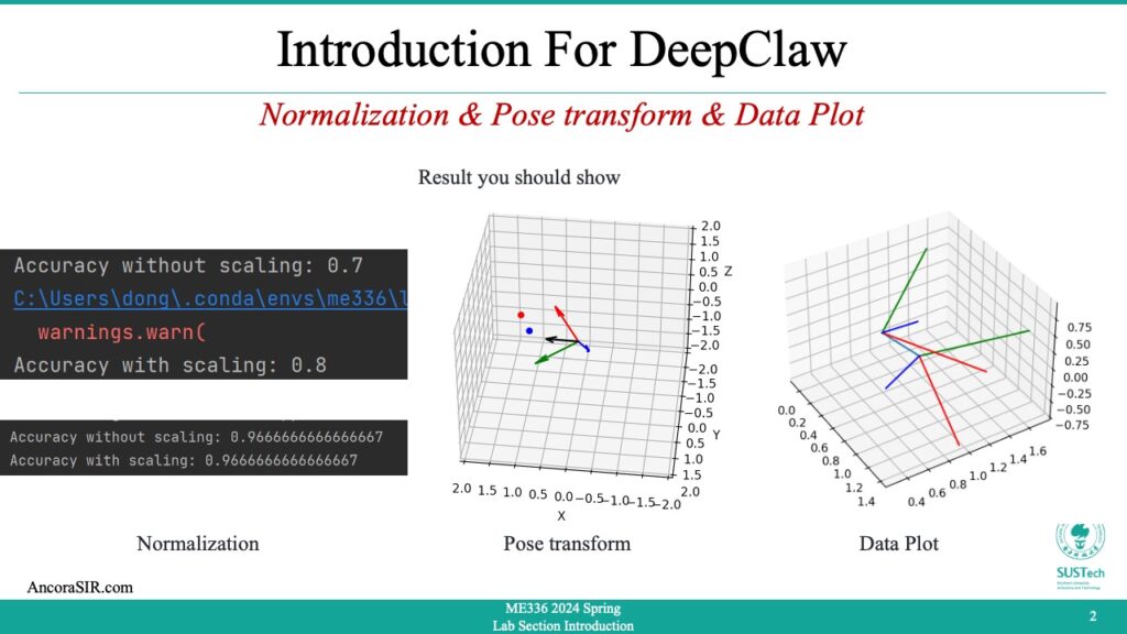
pip install matplotlibTask 1: Normalization
- Normalization in machine learning is the process of rescaling the feature values of a dataset to a common scale. The goal of normalization is to bring all the features on a level playing field, so that none of them dominates the others. This is particularly important when working with datasets where the features have different units of measurement or different ranges.
- There are several methods of normalization, but the most common ones are:
- Min-max normalization: This involves rescaling the feature values to a range of 0 to 1. The formula for min-max normalization is:
xnormalized = (x - xmin) / (xmax - xmin)where x is the original value of the feature, xmin is the minimum value of the feature in the dataset, and xmax is the maximum value of the feature in the dataset. - Z-score normalization: This involves rescaling the feature values so that they have a mean of 0 and a standard deviation of 1. The formula for z-score normalization is:
xnormalized = (x - mean) / SDwhere x is the original value of the feature, mean is the mean value of the feature in the dataset, and SD is the standard deviation of the feature in the dataset.
- Min-max normalization: This involves rescaling the feature values to a range of 0 to 1. The formula for min-max normalization is:
- Normalization is an important preprocessing step in machine learning, as it can improve the performance of many algorithms, especially those that are sensitive to the scale of the features and code in right shows the process for Min-max normalization.
Min-max normalization
from sklearn.neural_network import MLPClassifier
from sklearn.datasets import load_iris
from sklearn.model_selection import train_test_split
from sklearn.preprocessing import MinMaxScaler

# Load the iris dataset
iris = load_iris()

# Split the data into training and test sets
X_train, X_test, y_train, y_test = train_test_split(
    iris.data, iris.target, test_size=0.2, random_state=42)

# Create an MLP without scaling the data
mlp_no_scaling = MLPClassifier(hidden_layer_sizes=(10,), max_iter=200, random_state=42)
mlp_no_scaling.fit(X_train, y_train)

# Evaluate the MLP without scaling
score_no_scaling = mlp_no_scaling.score(X_test, y_test)
print(f"Accuracy without scaling: {score_no_scaling}")

# Create an MLP with scaling the data between 0 and 1
scaler = MinMaxScaler()
X_train_scaled = scaler.fit_transform(X_train)
X_test_scaled = scaler.transform(X_test)

mlp_scaling = MLPClassifier(hidden_layer_sizes=(10,), max_iter=200, random_state=42)
mlp_scaling.fit(X_train_scaled, y_train)

# Evaluate the MLP with scaling
score_scaling = mlp_scaling.score(X_test_scaled, y_test)
print(f"Accuracy with scaling: {score_scaling}")
Task 2: Pose transform
- Rotation vector and rotation matrix are both mathematical representations used to describe the orientation or rotation of an object in 3D space.
- A rotation vector is a compact representation of a 3D rotation that represents the axis of rotation and the amount of rotation around that axis. It is typically represented as a 3-element vector whose direction defines the axis of rotation, and whose magnitude represents the amount of rotation in radians. The rotation vector can be converted to a rotation matrix, which is a more common representation of a rotation.
- A rotation matrix is a 3×3 matrix that describes a rotation in 3D space. Each column of the matrix represents the direction of one of the transformed coordinate axes, and the elements of the column represent the components of the new basis vectors in terms of the original basis vectors. A rotation matrix can be used to transform a point or vector from one coordinate system to another that is rotated with respect to the original coordinate system.
- Both rotation vectors and rotation matrices are commonly used in computer graphics, robotics, and other fields that involve working with 3D data. They can be used to represent the orientation of objects, animate movements, and transform 3D data between different coordinate systems.
- In this code sample, we first define a rotation angle and axis using the
thetaandaxisvariables. We then construct the corresponding rotation matrixR. - Next, we generate a set of points using
numpy.random.normaland apply the rotation matrix to them usingnumpy.dot. The resulting set of rotated points is stored inrotated_points. - Finally, using Matplotlib’s
scatterfunction to plot the original and rotated points in 3D space. The original points are shown in blue, while the rotated points are shown in red, the axis of rotation as a vector in the same 3D plot represents the new coordinate system after the rotation.
Python
import numpy as np
import matplotlib.pyplot as plt
from mpl_toolkits.mplot3d import Axes3D

# Define rotation angle and axis
theta = np.pi/4  # 45 degrees
axis = np.array([1, 1, 1]) / np.sqrt(3)  # unit vector along diagonal axis

# Construct rotation matrix
c = np.cos(theta)
s = np.sin(theta)
t = 1 - c
x, y, z = axis
R = np.array([[t*x*x + c, t*x*y - z*s, t*x*z + y*s],
              [t*x*y + z*s, t*y*y + c, t*y*z - x*s],
              [t*x*z - y*s, t*y*z + x*s, t*z*z + c]])

# Plot transformed basis vectors
x_axis = np.dot(R, np.array([1, 0, 0]))
y_axis = np.dot(R, np.array([0, 1, 0]))
z_axis = np.dot(R, np.array([0, 0, 1]))

# Define set of points to rotate
n_points = 1
points = np.random.normal(size=(n_points, 3))

# Apply rotation matrix to points
rotated_points = np.dot(R, points.T).T

# Visualize original and rotated points
fig = plt.figure()
ax = fig.add_subplot(111, projection='3d')
ax.quiver(0, 0, 0, x_axis[0], x_axis[1], x_axis[2], color='red')
ax.quiver(0, 0, 0, y_axis[0], y_axis[1], y_axis[2], color='green')
ax.quiver(0, 0, 0, z_axis[0], z_axis[1], z_axis[2], color='blue')
ax.scatter(points[:,0], points[:,1], points[:,2], color='blue')
ax.scatter(rotated_points[:,0], rotated_points[:,1], rotated_points[:,2], color='red')

# Plot axis of rotation
ax.quiver(0, 0, 0, axis[0], axis[1], axis[2], color='black')

ax.set_xlim(-2, 2)
ax.set_ylim(-2, 2)
ax.set_zlim(-2, 2)
ax.set_xlabel('X')
ax.set_ylabel('Y')
ax.set_zlabel('Z')
plt.show()
Task 3: Data Plot
- This code generates a 3D plot with orientation information for a 6-dimensional motion data. It uses the Matplotlib and NumPy libraries.
- First, it imports Matplotlib and NumPy with the aliases “plt” and “np”, respectively.
- Then, it generates a 4×6 NumPy array “data” with random values between 0 and 1.
- The function “plot_motion_6d” takes the “data” array and a boolean parameter “draw_rpy” as input. It splits the data into x, y, z, roll, pitch, and yaw variables using NumPy slicing.
- Next, it creates a new 3D figure using Matplotlib and adds a subplot to it with the “projection=’3d'” argument.
- Then, it plots the x, y, and z variables in the subplot using the “ax.plot” function.
- If the “draw_rpy” parameter is True, the function adds orientation information to the plot. For each row in the data array, it calculates a 3×3 rotation matrix using the roll, pitch, and yaw values. It then calculates the end points of three vectors corresponding to the rotation matrix and plots them in red, green, and blue colors using the “ax.plot” function.
Python
import matplotlib.pyplot as plt
import numpy as np

# Generate sample data
data = np.random.rand(4, 6)

def plot_motion_6d(data, draw_rpy=True):
    # Split data into x, y, z, roll, pitch, and yaw
    x = data[:, 0]
    y = data[:, 1]
    z = data[:, 2]
    roll = data[:, 3]
    pitch = data[:, 4]
    yaw = data[:, 5]

    # Plot data in 3D
    fig = plt.figure()
    ax = fig.add_subplot(111, projection='3d')
    ax.plot(x, y, z)

    # Add orientation information
    if draw_rpy:
        for i in range(len(data)):
            R = np.array([[np.cos(yaw[i])*np.cos(pitch[i]), np.cos(yaw[i])*np.sin(pitch[i])*np.sin(roll[i]) - np.sin(yaw[i])*np.cos(roll[i]), np.cos(yaw[i])*np.sin(pitch[i])*np.cos(roll[i]) + np.sin(yaw[i])*np.sin(roll[i])],
                          [np.sin(yaw[i])*np.cos(pitch[i]), np.sin(yaw[i])*np.sin(pitch[i])*np.sin(roll[i]) + np.cos(yaw[i])*np.cos(roll[i]), np.sin(yaw[i])*np.sin(pitch[i])*np.cos(roll[i]) - np.cos(yaw[i])*np.sin(roll[i])],
                          [-np.sin(pitch[i]), np.cos(pitch[i])*np.sin(roll[i]), np.cos(pitch[i])*np.cos(roll[i])]])
            x_end = x[i] + R[0, 0]
            y_end = y[i] + R[1, 0]
            z_end = z[i] + R[2, 0]
            ax.plot([x[i], x_end], [y[i], y_end], [z[i], z_end], 'r')
            x_end = x[i] + R[0, 1]
            y_end = y[i] + R[1, 1]
            z_end = z[i] + R[2, 1]
            ax.plot([x[i], x_end], [y[i], y_end], [z[i], z_end], 'g')
            x_end = x[i] + R[0, 2]
            y_end = y[i] + R[1, 2]
            z_end = z[i] + R[2, 2]
            ax.plot([x[i], x_end], [y[i], y_end], [z[i], z_end], 'b')

    plt.show()

plot_motion_6d(data,draw_rpy=True)
Task 4: Kalman filter
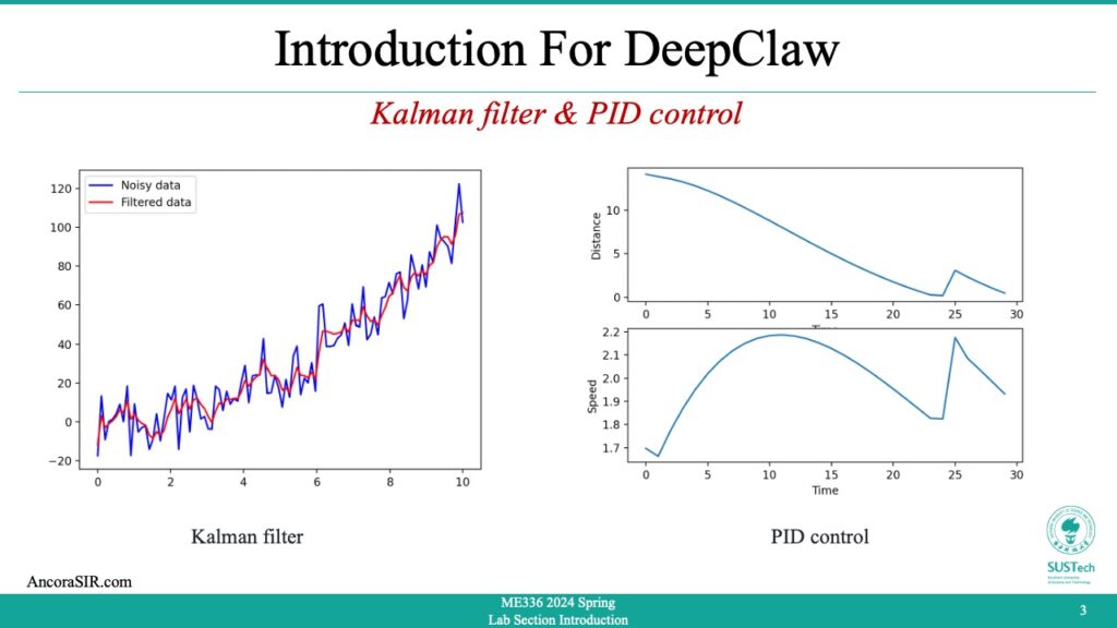
- Kalman refers to the Kalman filter, a mathematical algorithm used for estimation and prediction of a system’s state. It is widely used in control and signal processing applications, particularly in aerospace, navigation, and robotics. The algorithm uses a series of measurements over time to estimate the current state of a system and predict its future behavior. The Kalman filter is named after its developer, Rudolf Kalman, who published the initial paper on the filter in 1960.
- This code demonstrates an implementation of the Kalman filter to filter noisy data. Here’s a step-by-step explanation:
- Generate some noisy data for the function y = x^2. The input x is generated using
np.linspaceto create 100 evenly spaced values between 0 and 10. The noise is added usingnp.random.normal, with a mean of 0 and a standard deviation of 10. - Initialize the Kalman filter with some initial values.
x_hatis the initial state estimate, initialized to a 2D vector of zeros.Pis the initial estimate of the error covariance matrix, initialized to a diagonal matrix with large values on the diagonal to reflect high uncertainty.Fis the state transition matrix, which predicts the next state based on the current state, initialized as a 2×2 matrix.Qis the process noise covariance matrix, which models the uncertainty in the process that generates the state, initialized as a diagonal matrix.His the measurement matrix, which maps the state estimate to the measurement space, initialized as a 1×2 matrix.Ris the measurement noise covariance matrix, which models the uncertainty in the measurement, initialized as a 1×1 matrix. - Apply the Kalman filter to the noisy data. For each data point, predict the next state based on the previous state estimate and the state transition matrix. Update the state estimate based on the measurement, using the Kalman gain matrix to balance the information from the prediction and the measurement. Append the filtered measurement to the
filtered_ylist. - Sort the noisy data points by x value, and plot the original noisy data as a blue line and the filtered data as a red line using
plt.plot. Add a legend and show the plot usingplt.legendandplt.show. - Install
matplotlibbypip install matplotlibin your python environment.
Python
import numpy as np
import matplotlib.pyplot as plt
from mpl_toolkits.mplot3d import Axes3D

# Generate noisy data from the function y=x^2
x = np.linspace(0, 10, 100)
noise = np.random.normal(loc=0, scale=10, size=100)
y = x**2 + noise

# Initialize the Kalman filter
x_hat = np.zeros(2)
P = np.diag([100, 100])
F = np.array([[1, 1], [0, 1]])
Q = np.diag([1, 1])
H = np.array([1, 0]).reshape(1, 2)
R = np.array([100]).reshape(1, 1)

# Apply the Kalman filter to the noisy data
filtered_y = []
for i in range(len(x)):
    # Predict the next state
    x_hat = F.dot(x_hat)
    P = F.dot(P).dot(F.T) + Q

    # Update the state estimate based on the measurement
    y_hat = H.dot(x_hat)
    K = P.dot(H.T).dot(np.linalg.inv(H.dot(P).dot(H.T) + R))
    x_hat = x_hat + K.dot(y[i] - y_hat)
    P = (np.eye(2) - K.dot(H)).dot(P)

    filtered_y.append(H.dot(x_hat))

# Connect the noisy data points in order
noisy_data = np.column_stack((x, y))
sorted_noisy_data = noisy_data[noisy_data[:,0].argsort()]

# Plot the original noisy data and the filtered data
plt.plot(sorted_noisy_data[:,0], sorted_noisy_data[:,1], 'b-', label='Noisy data')
plt.plot(x, filtered_y, 'r-', label='Filtered data')
plt.legend()
plt.show()
Task 5: PID control
- PID control is a technique used in control systems to adjust the behavior of a system by calculating an error signal and using it to adjust an input signal. The acronym PID stands for Proportional-Integral-Derivative, which refers to the three types of control actions used in a PID controller.
- The proportional term adjusts the input signal proportionally to the error signal, which is the difference between the desired output and the actual output of the system. The integral term adjusts the input signal based on the accumulated error over time, which helps to eliminate steady-state errors. The derivative term adjusts the input signal based on the rate of change of the error signal, which helps to reduce overshoot and stabilize the system.
- PID controllers are widely used in various fields, such as industrial control, robotics, and automation. They are effective in controlling systems that have a dynamic response, and can be used to regulate temperature, pressure, speed, and other parameters.
- In the sample code simulates a simple example of a PID controller controlling the velocity of point A (represented by x1 and y1) in order to reach point B (represented by x2 and y2). The distance between the two points is used as the error signal in the PID controller, and the output of the controller is used to control the velocity of point A.
- The simulation loop runs for 100 time steps, and on each iteration it calculates the distance between the two points, checks if they have met, calculates the error between the distance and the desired value (which is 0 in this case), calculates the P, I, and D terms of the PID controller, calculates the output of the controller, limits the output to a maximum velocity, updates the velocity of point A based on the output of the controller, and updates the positions of both points based on their velocities.
- During the simulation loop, the code also records data about the time, distance, and speed at each time step, and plots the results in two subplots using Matplotlib. The first subplot shows the distance between the two points over time, while the second subplot shows the speed of point A over time.
Python
import math

# PID constants
Kp = 0.1
Ki = 0.01
Kd = 0.01

# Initial positions and velocities
x1, y1 = 0, 0
vx1, vy1 = 0, 0
x2, y2 = 10, 10
vx2, vy2 = 1, 1

# PID variables
error_sum = 0
last_error = 0

# Lists for storing data
times = []
distances = []
speeds = []

# Simulation loop
for t in range(100):
    # Calculate distance between points
    dx = x2 - x1
    dy = y2 - y1
    distance = math.sqrt(dx * dx + dy * dy)

    # Check if points have met
    if distance < 0.1:
        break

    # Calculate error and PID terms
    error = distance
    error_sum += error
    delta_error = error - last_error
    last_error = error

    P = Kp * error
    I = Ki * error_sum
    D = Kd * delta_error

    # Calculate PID output
    output = P + I + D

    # Limit output to maximum velocity
    max_speed = 100
    if output > max_speed:
        output = max_speed
    elif output < -max_speed:
        output = -max_speed

    # Update velocity of point A
    vx1 = output * dx / distance
    vy1 = output * dy / distance

    # Update position of points
    x1 += vx1
    y1 += vy1
    x2 += vx2
    y2 += vy2

    # Record data
    times.append(t)
    distances.append(distance)
    speeds.append(output)

# Plot results
import matplotlib.pyplot as plt

plt.subplot(2, 1, 1)
plt.plot(times, distances)
plt.xlabel('Time')
plt.ylabel('Distance')

plt.subplot(2, 1, 2)
plt.plot(times, speeds)
plt.xlabel('Time')
plt.ylabel('Speed')

plt.show()
Task 6: Action Feedback and Control
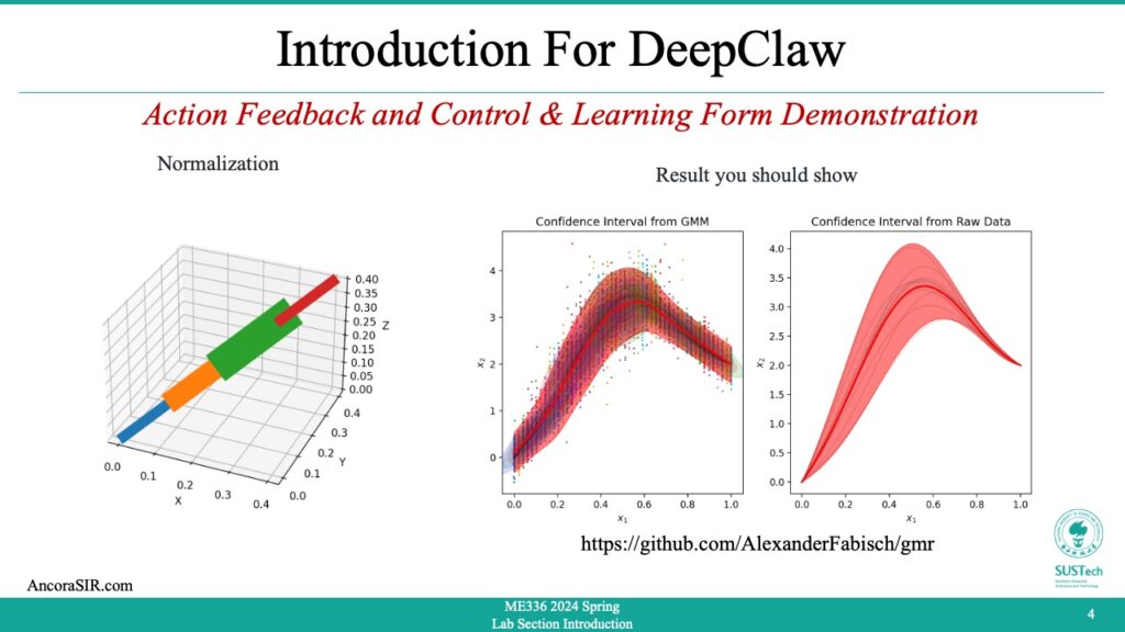
- This code creates a 3D plot of a motion curve, where the thickness of the line connecting the points is based on the magnitude of the corresponding force.
- The x, y, and z coordinates of the motion data are stored in the lists
x,y, andz, respectively, and the magnitudes of the corresponding forces are stored in the listforce_mag.
- The code creates a 3D plot using
matplotlib‘sAxes3Dmodule and sets up a subplot with a 3D projection. Then, for each pair of adjacent points in the motion data, the code plots a line connecting those two points with a linewidth proportional to the corresponding force magnitude. Theforloop iterates over the range of the length ofxminus one, since the last point in the motion data has no line connecting it to another point.
Python
import numpy as np
import matplotlib.pyplot as plt
from mpl_toolkits.mplot3d import Axes3D


# Extract the x, y, and z coordinates from the motion data and force_mag for the Normal Force
x = [0,0.1,0.2,0.3,0.4]
y = [0,0.1,0.2,0.3,0.4]
z = [0,0.1,0.2,0.3,0.4]

force_mag= [1, 2, 3, 1]
# Set up the 3D plot and adjust the thickness of the line based on the force data
fig = plt.figure()
ax = fig.add_subplot(111, projection='3d')
for i in range(len(x)-1):
    ax.plot(x[i:i+2], y[i:i+2], z[i:i+2], linewidth=force_mag[i]*10)

# Add labels and a title to the plot
ax.set_xlabel('X')
ax.set_ylabel('Y')
ax.set_zlabel('Z')
ax.set_title('3D Motion Curve with Force Magnitude')

# Show the plot
plt.show()
Class 2 in Week 07 Fri
GMR(Gaussian Mixture Regression)
- Gaussian mixture regression is a statistical technique used to model the relationship between a set of independent variables and a continuous dependent variable. It assumes that the dependent variable is a linear combination of several Gaussian distributions (i.e., normal distributions) with different means and variances.
- In other words, Gaussian mixture regression assumes that the data comes from several subpopulations, each with its own Gaussian distribution. These subpopulations can be modeled using a mixture of Gaussians, which is a weighted sum of several Gaussian distributions.
- To estimate the parameters of the Gaussian mixture model, maximum likelihood estimation is often used. This involves finding the values of the means, variances, and weights of the Gaussian distributions that maximize the likelihood of observing the data.
- Once the Gaussian mixture model is estimated, it can be used to predict the value of the dependent variable for new observations based on the values of the independent variables. The prediction is based on the probability density function of the mixture model, which gives the probability of observing a particular value of the dependent variable given the values of the independent variables.
- Gaussian mixture regression is often used in cases where the relationship between the independent and dependent variables is nonlinear and cannot be captured by a simple linear regression model. It is also useful in cases where the data may have multiple underlying distributions, which can be modeled using a mixture of Gaussians.
Python
from sklearn.mixture import GaussianMixture
import numpy as np

# create example data
x = np.random.rand(100, 2) * 10
y = np.sin(x[:, 0]) + np.cos(x[:, 1]) + np.random.normal(scale=0.5, size=100)

# create Gaussian mixture regression model
gmm = GaussianMixture(n_components=3)

# fit the model to the data
gmm.fit(x, y)

# predict the output for new input
x_new = np.array([[2, 2], [4, 4], [6, 6]])
y_new = gmm.predict(x_new)

print(y_new)
Action data collection
- This part is similar to Visual Object Tracking in session 1, except that this experiment captures action(motion+force) data in real time.
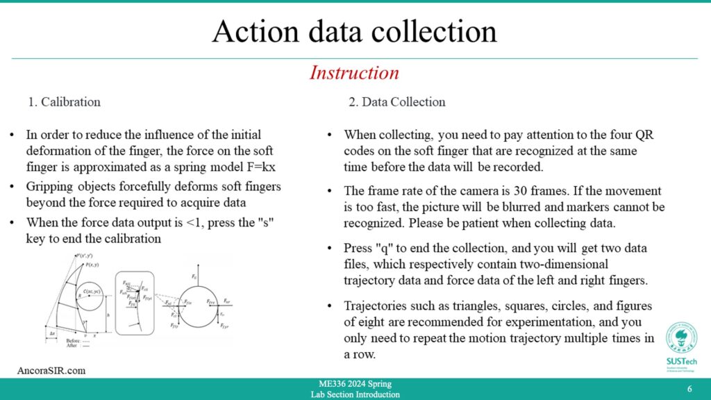
- In order to reduce the influence of the initial deformation of the finger, the force on the soft finger is approximated as a spring model F=kx.
- Gripping objects forcefully deforms soft fingers beyond the force required to acquire data.
- When the force data output is <1, press the “s” key to end the calibration.
- When collecting, you need to pay attention to the four QR codes on the soft finger that are recognized at the same time before the data will be recorded.
- The frame rate of the camera is 30 frames. If the movement is too fast, the picture will be blurred and markers cannot be recognized. Please be patient when collecting data.
- Press “q” to end the collection, and you will get two data files, which respectively contain two-dimensional trajectory data and force data of the left and right fingers.
- Trajectories such as triangles, squares, circles, and figures of eight are recommended for experimentation, and you only need to repeat the motion trajectory multiple times in a row.
Python
import cv2
import time
import numpy as np
import math
import cv2.aruco as aruco

aruco_dict = aruco.Dictionary_get(cv2.aruco.DICT_4X4_50)
aruco_params = aruco.DetectorParameters_create()
'''
If an error occurs, please use the following two lines of code.
如果报错,请将上面两行代码注释掉,用后面这两行代码
'''
# aruco_dict = aruco.getPredefinedDictionary(aruco.DICT_4X4_50)
# aruco_params = aruco.DetectorParameters()

aruco_params.cornerRefinementMethod = aruco.CORNER_REFINE_CONTOUR
# Initialize camera capture
cap = cv2.VideoCapture(0)
cap.set(cv2.CAP_PROP_FRAME_WIDTH, 1280)
cap.set(cv2.CAP_PROP_FRAME_HEIGHT, 720)
print(cap.get(3), cap.get(4), cap.get(5))

d23_min = 1
d45_min = 1
d23_max = 0
d45_max = 0
calibFlag = False
# Define an empty list to store the time series data
marker_poses = []

# Get the start time
start_time = time.time()

# Load the result from camera calibration
data = np.load('camera_params.npz')
mtx = data['mtx']
dist = data['dist']

force_left_finger = 0
force_right_finger = 0
midpointTvec = np.array([0, 0, 0])
trai_datas = []
trai_data = np.array([0, 0])  # x,y for the midPoint for marker 0,1
force_datas = []
force_data = np.array([0, 0])

# Play the video
while cap.isOpened():
    # Read the next frame
    ret, frame = cap.read()
    if ret == True:
        # Get the current time
        current_time = time.time()
        # Detect ArUco markers in the frame
        corners, ids, rejected = cv2.aruco.detectMarkers(frame, aruco_dict, parameters=aruco_params)
        if ids is not None:
            # Loop over all detected markers
            rvecs, tvecs, _objPoints = cv2.aruco.estimatePoseSingleMarkers(corners, 0.05, mtx, dist)
            for i in range(0, ids.size):
                # draw axis for the aruco markers
                cv2.drawFrameAxes(frame, mtx, dist, rvecs[i], tvecs[i], 0.1)
            if 2 in ids and 3 in ids:
                marker2_idx = np.where(ids == 2)[0][0]
                marker3_idx = np.where(ids == 3)[0][0]

                t2 = tvecs[marker2_idx].reshape(-1)
                t3 = tvecs[marker3_idx].reshape(-1)
                d23 = math.sqrt((t2[0] - t3[0]) ** 2 + (t2[1] - t3[1]) ** 2)
                if d23 < d23_min:
                    d23_min = d23
                    force_left_finger = 0
                elif d23 > d23_max:
                    d23_max = d23
                    force_left_finger = 1
                else:
                    force_left_finger = (d23 - d23_min) / (d23_max - d23_min)

            if 4 in ids and 5 in ids:
                marker4_idx = np.where(ids == 4)[0][0]
                marker5_idx = np.where(ids == 5)[0][0]

                t4 = tvecs[marker4_idx].reshape(-1)
                t5 = tvecs[marker5_idx].reshape(-1)
                d45 = math.sqrt((t4[0] - t5[0]) ** 2 + (t4[1] - t5[1]) ** 2)
                if d45 < d45_min:
                    d45_min = d45
                    force_right_finger = 0
                elif d45 > d45_max:
                    d45_max = d45
                    force_right_finger = 1
                else:
                    force_right_finger = (d45 - d45_min) / (d45_max - d45_min)

            if 3 in ids and 5 in ids:
                marker3_idx = np.where(ids == 3)[0][0]
                marker5_idx = np.where(ids == 5)[0][0]
                midpointTvec = ((tvecs[marker3_idx] + tvecs[marker5_idx]) / 2)[0]
                # print(midpointTvec)

            if 2 in ids and 3 in ids and 4 in ids and 5 in ids:
                print("Force:",force_left_finger,force_right_finger)
                if calibFlag:
                    traj_data = np.array([midpointTvec[0], midpointTvec[1]])
                    trai_datas.append(traj_data)
                    force_data = np.array([force_left_finger, force_right_finger])
                    force_datas.append(force_data)

            # Display the frame
            cv2.imshow('Frame', frame)
            # Exit on key press
            if cv2.waitKey(1) & 0xFF == ord('s'):
                calibFlag = True
                print("Start Collection...")
            if cv2.waitKey(1) & 0xFF == ord('q'):
                break

            # Wait for the specified delay (in milliseconds)
            cv2.waitKey(1)
        else:
            break
print(len(trai_datas))
print(len(force_datas))

np.save('trajdataForLFD.npy', trai_datas)
np.save('forcedataForLFD.npy', force_datas)

# Release the video capture and destroy all windows
cap.release()
cv2.destroyAllWindows()
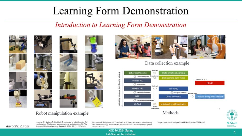
Learning From Demonstration
- This is a Python code for generating and plotting noisy trajectories for testing imitation learning. It also includes Gaussian Mixture Model (GMM) for the generated trajectories and conditions the GMM to predict the mean and covariance of the trajectory at each time step.
- Defining a function
make_demonstrationsthat generatesn_demonstrationsnoisy demonstrations withn_stepstime steps each. The function takes several optional parameters includingsigmaandmuto specify the standard deviation and mean of the noisy component,startandgoalto specify the initial and final positions of the trajectory, andrandom_stateto set a seed for the random number generator. The function returns two arraysXandground_truth.Xis a 3D array of shape(n_task_dims, n_steps, n_demonstrations)containing the noisy demonstrated trajectories.ground_truthis a 2D array of shape(n_task_dims, n_steps)containing the original trajectory.
Python
import numpy as np
import matplotlib.pyplot as plt
from matplotlib.patches import Ellipse
from sklearn.mixture import BayesianGaussianMixture
from itertools import cycle
from gmr import GMM, kmeansplusplus_initialization, covariance_initialization
from gmr.utils import check_random_state


def make_demonstrations(n_demonstrations, n_steps, sigma=0.25, mu=0.5,
                        start=np.zeros(2), goal=np.ones(2), random_state=None):
    """Generates demonstration that can be used to test imitation learning.
    Parameters
    ----------
    n_demonstrations : int
        Number of noisy demonstrations
    n_steps : int
        Number of time steps
    sigma : float, optional (default: 0.25)
        Standard deviation of noisy component
    mu : float, optional (default: 0.5)
        Mean of noisy component
    start : array, shape (2,), optional (default: 0s)
        Initial position
    goal : array, shape (2,), optional (default: 1s)
        Final position
    random_state : int
        Seed for random number generator
    Returns
    -------
    X : array, shape (n_task_dims, n_steps, n_demonstrations)
        Noisy demonstrated trajectories
    ground_truth : array, shape (n_task_dims, n_steps)
        Original trajectory
    """
    random_state = np.random.RandomState(random_state)

    X = np.empty((2, n_steps, n_demonstrations))

    # Generate ground-truth for plotting
    ground_truth = np.empty((2, n_steps))
    T = np.linspace(-0, 1, n_steps)
    ground_truth[0] = T
    ground_truth[1] = (T / 20 + 1 / (sigma * np.sqrt(2 * np.pi)) *
                       np.exp(-0.5 * ((T - mu) / sigma) ** 2))

    # Generate trajectories
    for i in range(n_demonstrations):
        noisy_sigma = sigma * random_state.normal(1.0, 0.1)
        noisy_mu = mu * random_state.normal(1.0, 0.1)
        X[0, :, i] = T
        X[1, :, i] = T + (1 / (noisy_sigma * np.sqrt(2 * np.pi)) *
                          np.exp(-0.5 * ((T - noisy_mu) /
                                         noisy_sigma) ** 2))

    # Spatial alignment
    current_start = ground_truth[:, 0]
    current_goal = ground_truth[:, -1]
    current_amplitude = current_goal - current_start
    amplitude = goal - start
    ground_truth = ((ground_truth.T - current_start) * amplitude /
                    current_amplitude + start).T

    for demo_idx in range(n_demonstrations):
        current_start = X[:, 0, demo_idx]
        current_goal = X[:, -1, demo_idx]
        current_amplitude = current_goal - current_start
        X[:, :, demo_idx] = ((X[:, :, demo_idx].T - current_start) *
                             amplitude / current_amplitude + start).T

    return X, ground_truth


plot_covariances = True
X, _ = make_demonstrations(
    n_demonstrations=10, n_steps=50, goal=np.array([1., 2.]),
    random_state=0)
X = X.transpose(2, 1, 0)
steps = X[:, :, 0].mean(axis=0)
expected_mean = X[:, :, 1].mean(axis=0)
expected_std = X[:, :, 1].std(axis=0)

n_demonstrations, n_steps, n_task_dims = X.shape
X_train = np.empty((n_demonstrations, n_steps, n_task_dims + 1))
X_train[:, :, 1:] = X
t = np.linspace(0, 1, n_steps)
X_train[:, :, 0] = t
X_train = X_train.reshape(n_demonstrations * n_steps, n_task_dims + 1)

random_state = check_random_state(0)
n_components = 4
initial_means = kmeansplusplus_initialization(X_train, n_components, random_state)
initial_covs = covariance_initialization(X_train, n_components)
bgmm = BayesianGaussianMixture(n_components=n_components, max_iter=100).fit(X_train)
gmm = GMM(
    n_components=n_components,
    priors=bgmm.weights_,
    means=bgmm.means_,
    covariances=bgmm.covariances_,
    random_state=random_state)

plt.figure(figsize=(10, 5))
plt.subplot(121)
plt.title("Confidence Interval from GMM")

plt.plot(X[:, :, 0].T, X[:, :, 1].T, c="k", alpha=0.1)

means_over_time = []
y_stds = []
for step in t:
    conditional_gmm = gmm.condition([0], np.array([step]))
    conditional_mvn = conditional_gmm.to_mvn()
    means_over_time.append(conditional_mvn.mean)
    y_stds.append(np.sqrt(conditional_mvn.covariance[1, 1]))
    samples = conditional_gmm.sample(100)
    plt.scatter(samples[:, 0], samples[:, 1], s=1)
means_over_time = np.array(means_over_time)
y_stds = np.array(y_stds)

plt.plot(means_over_time[:, 0], means_over_time[:, 1], c="r", lw=2)
plt.fill_between(
    means_over_time[:, 0],
    means_over_time[:, 1] - 1.96 * y_stds,
    means_over_time[:, 1] + 1.96 * y_stds,
    color="r", alpha=0.5)

if plot_covariances:
    colors = cycle(["r", "g", "b"])
    for factor in np.linspace(0.5, 4.0, 8):
        new_gmm = GMM(
            n_components=len(gmm.means), priors=gmm.priors,
            means=gmm.means[:, 1:], covariances=gmm.covariances[:, 1:, 1:],
            random_state=gmm.random_state)
        for mean, (angle, width, height) in new_gmm.to_ellipses(factor):
            ell = Ellipse(xy=mean, width=width, height=height,
                            angle=np.degrees(angle))
            ell.set_alpha(0.15)
            ell.set_color(next(colors))
            plt.gca().add_artist(ell)

plt.xlabel("$x_1$")
plt.ylabel("$x_2$")

plt.subplot(122)
plt.title("Confidence Interval from Raw Data")
plt.plot(X[:, :, 0].T, X[:, :, 1].T, c="k", alpha=0.1)

plt.plot(steps, expected_mean, c="r", lw=2)
plt.fill_between(
    steps,
    expected_mean - 1.96 * expected_std,
    expected_mean + 1.96 * expected_std,
    color="r", alpha=0.5)

plt.xlabel("$x_1$")
plt.ylabel("$x_2$")

plt.show()
Report Requirement for Tutorial Session in Week 07
For Part 1
- As a team, you need to record the experiment’s results in this part of the report. Since the code has been provided, you only need to modify the code parameters, take a screenshot, and fill in the blanks in the report template.
For Part 2 Reference Code
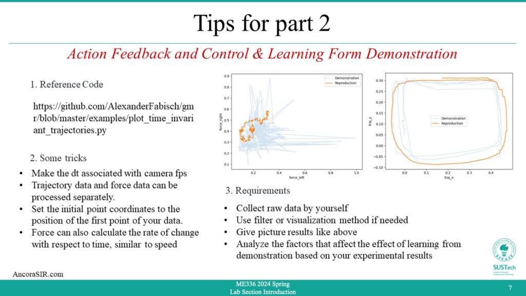
- As a team, your assignment is to use the DeepClaw toolkit to collect action data (motion + force/torque) for a specific manipulation task, visualize and analyze the collected data, and train a model to learn the action with the highest performance.
- The experiment setup for collecting the raw dataset is as follows: Fit the soft fingers to the jaws to complete the bracket assembly so that the camera is facing down.
- The data collection procedure is as follows: Use your hand to complete a trace (such as a letter) with the gripper gripping the force doll, and pay attention to controlling the strength of the grip. Complete the same task at least three times and collect data on actions (movement + force).
- Use the Gaussian method to learn these data, give the fitting results and analyze them
Report Template
- Please download the template and complete it according to the guidelines.
Files Needed
- The report should be in PDF format and renamed with your team number (example Team1-Lab2-Report.pdf).
- Only the code files you use in Class 2 need to be submitted and named properly
- All files are finally compressed into a zip file for submission and renamed with your team number (example Team1-Lab2.zip)